CMU 10601 的课程笔记。EM 算法计算含有隐含变量的概率模型参数估计,能使用在一些无监督的聚类方法上。在 EM 算法总结提出以前就有该算法思想的方法提出,例如 HMM 中用的 Baum-Welch 算法。
Graphical Models
Key idea
- Conditional independence assumptions useful (but Naive Bayes is extrem)
- Probabilistic graphical models are a joint probability distribution defined over a graph
Two types of graphical models:
- Directed graphs (Bayesian Networks)
- Undirected graphs (Markov Random Fields)
hard bias:
Distribution shares conditional independent assumptions
Independence
Marginal Independence
Definition: X is marginally independent of Y if
$$(\forall i,j)P(X=x_i,Y=y_j)=P(X=x_i)P(Y=y_j)$$
变种:
$(\forall i,j)P(X=x_i|Y=y_j)=P(X=x_i)$
$(\forall i,j)P(Y=y_j|X=x_i)=P(Y=y_j)$
Conditional Independence
Definition: X is conditional independent of Y given Z, if the probability distribution governing X is independent of the value of Y, given the value of Z
$$(\forall i,j,k)P(X=x_i|Y=y_j|Z=z_k)=P(X=x_i|Z=z_k)$$
即
$$P(X|Y,Z)=P(X|Z)$$
DGM(Directed Graphical Models)
DGM = Bayes Nets = Bayes Belief Networks
Directed graph = (potentially very large) set of conditional independent assumptions = factorization of joint probability(Likelihood function)
Bayesian Networks
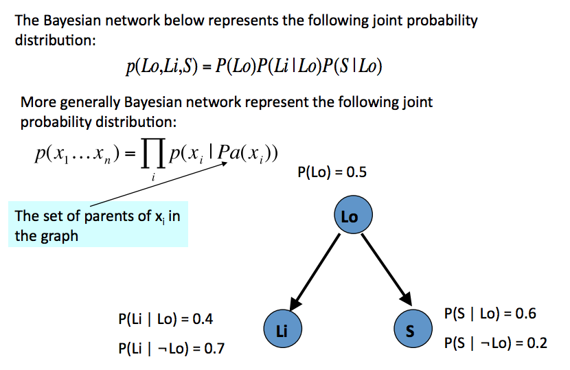
Causality
Causality => DCM
cannot infer causality from DCM
eg. A->B->C or C->B->A gives same DCM $C \bot A|B => A \bot C|B$
Types of DGM
Eg. Chain of events
Cloudy -> Rain -> Wetgrass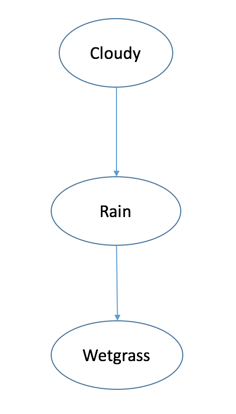
I(C;W)>=0
I(C;W|R)=0 $C \bot W|R$
Eg. Multiple Effects
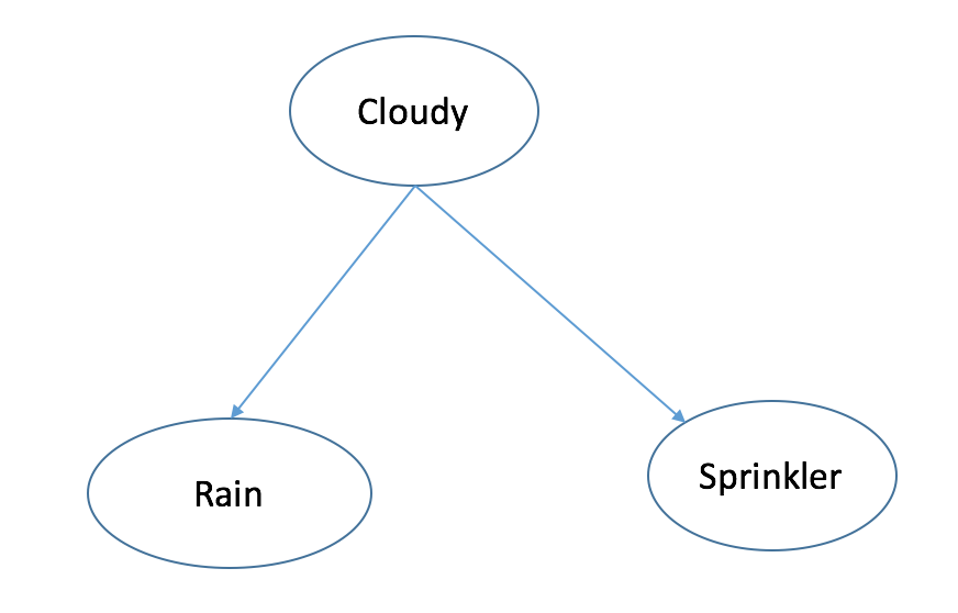
Cloudy -> Rain
-> Sprinkler
I(R;S)>=0 $R NOT \bot S$
I(R,S|C)=0 $R \bot S|C$
Eg. Multiple Causes
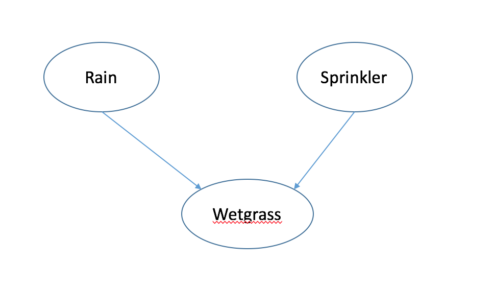
Rain -> Wetgrass
Sprinkler -> Wetgrass
I(R;S)=0 $R \bot S$
I(R,S|W)>=0 $R NOT \bot S|W$
“Explaining away”
look one of the factor explains the result
Factoring and Count parameters
Factoring 主要靠的是 chain rule 和 conditional independence assumptions,计算参数则主要看每个节点的父节点数。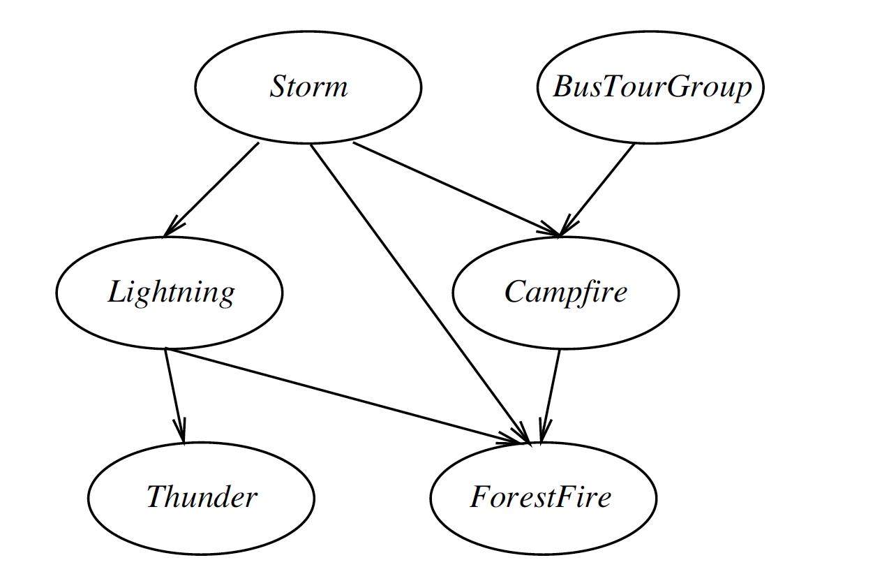
without independent Assumptions
P(S,B,L,C,T,F)=P(S)P(B|S)P(L|S,B)P(C|S,B,L)P(T|S,B,L,C)P(F|S,B,L,C,T)
# of paras 1+2+4+8+16+32
with these assumptions, condition only on immediate parent
=P(S)P(B)P(L|S)P(C|S,B)P(T|S,B)P(T|L)P(F|S,L,C)
# of paras 1+1+2+4+2+8=18
dominate factor: largest number of parents that any one node has
Example
再具体一点分析,假设我们有一个警报系统,有以下元素组成
Factoring joint distributions
12345P(M,J,A,B,E) =P(M |J,A,B,E) P(J,A,B,E) =P(M | J,A,B,E) P(J | A,B,E) P(A| B,E) =P(M | J,A,B,E) P(J | A,B,E) P(A | B,E) P(B,E)P(M | J,A,B,E) P(J | A,B,E) P(A | B,E)P(B | E)P(E)Draw Bayesian Network
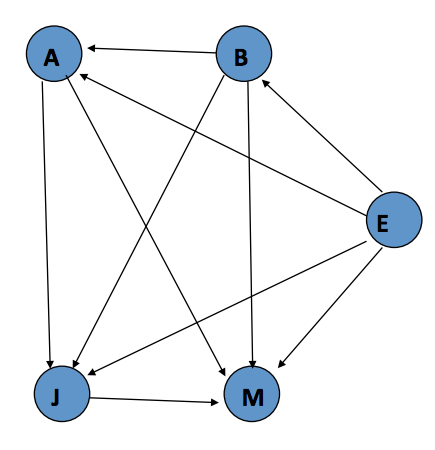
对上图来说,共需要 31 个参数。
M: 2^4
J: 2^3
A: 2^2
B: 2^1
E: 2^0- Use knowledge of domain
-> P(B)P(E)P(A|B,E)P(J|A)P(M|A)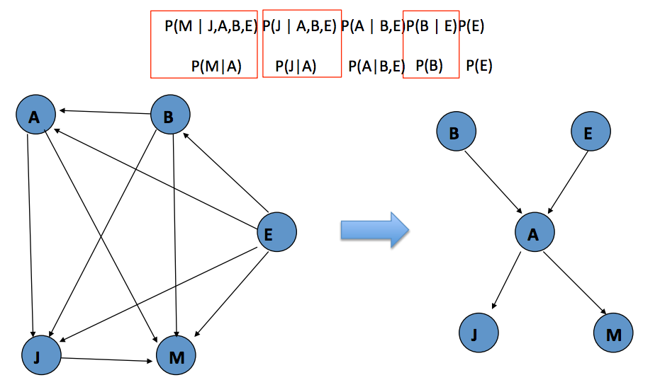 现在,需要 10 个参数(A:4, B:1, E:1, J:2, M:2),我们少用了 21 个参数!
Use
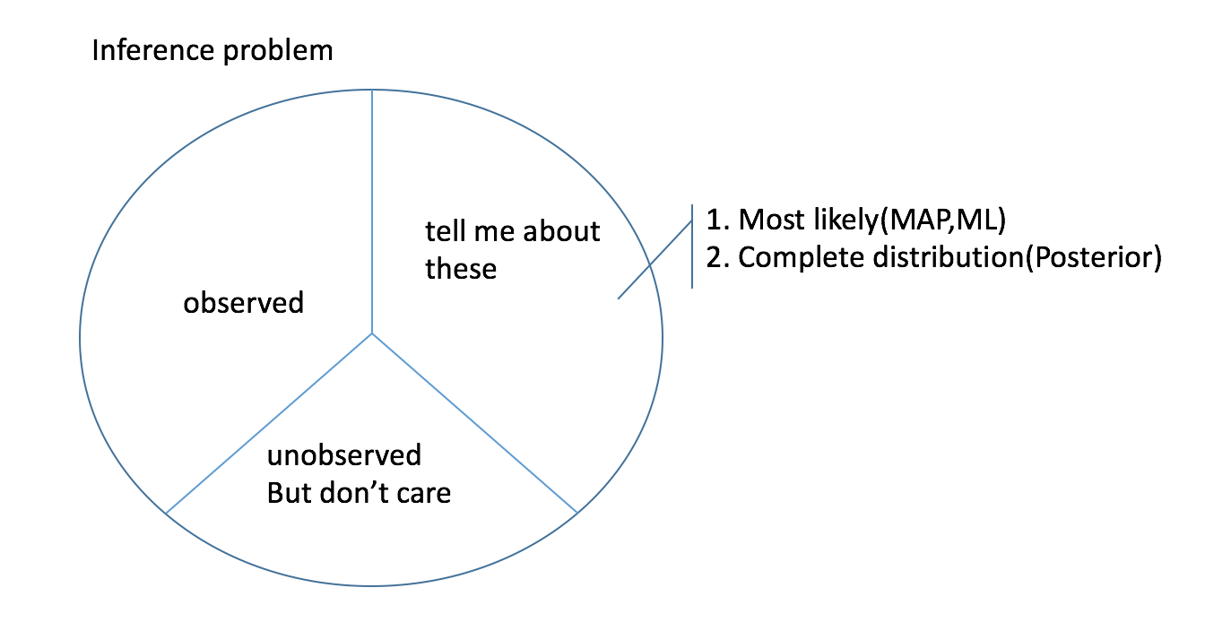
distribution posterior $P(Xt|Xo,\overline \theta)$
argmax $Xt = argmax \ P(Xt|Xo,\overline \theta)$
Using the model
Given the model (struct+params) input->output
Likelihood function twice
$P(X_k=0|X_1,..X_{k-1},X_{k+1}…X_p)$
$P(X_k=1|X_1,..X_{k-1},X_{k+1}…X_p)$
(if binary) normalize the two values, and gets the posterior
Condition on X1,X3,X5,X7
want to know: distribution over X2,X4,X6,X8
need to cal
$P(X_2=0,X_4=0,X_6=0,X_8=0,|X_1,..X_{k-1},X_{k+1}…X_p)$
$P(X_2=0,X_4=0,X_6=0,X_8=1,|X_1,..X_{k-1},X_{k+1}…X_p)$
…
$P(X_2=1,X_4=1,X_6=1,X_8=1,|X_1,..X_{k-1},X_{k+1}…X_p)$
cal all combinations, normalize, to get the posterior
exp(# of unobserved values)
Eg.1 Computing full joints
$P(B,\lnot E,A,J,\lnot M)$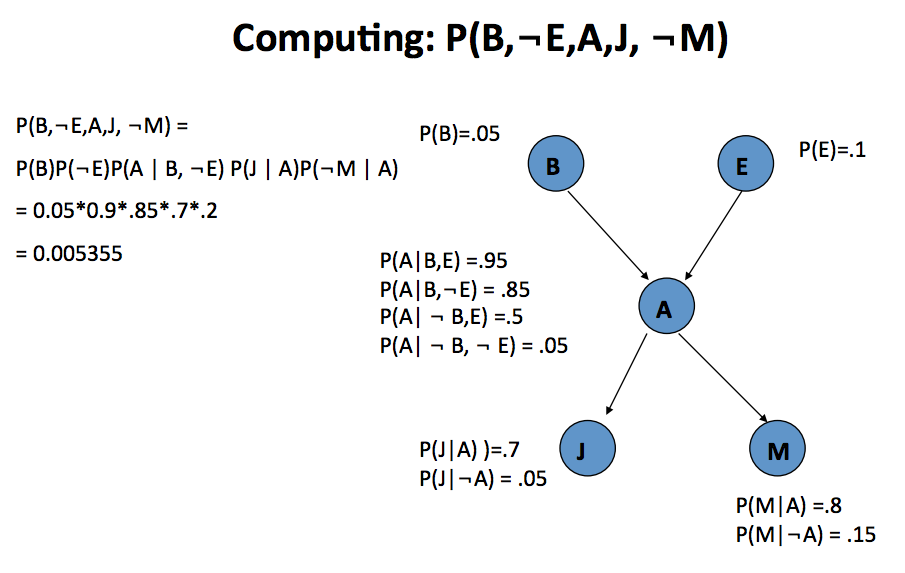
Eg.2 Compute partial joints
$P(B|J, \lnot M)$
$P(B|J, \lnot M)={P(B,J, \lnot M) \over P(B,J, \lnot M)+P(\lnot B,J,\lnot M)}$
Compute $P(B,J, \lnot M)$
Sum all instances with these settings (the sum is over the possible assignments to the other two variables, E and A)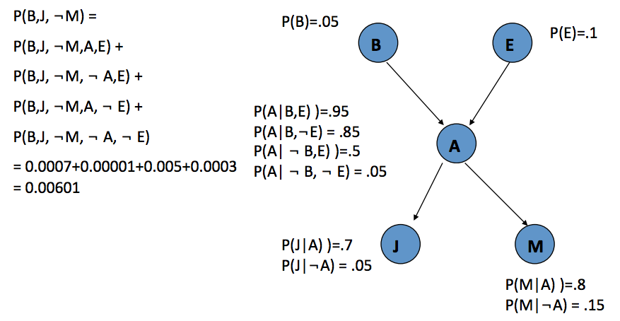
有简化的方法如 Variable elimination,这里不展开。
Things we do with regard to a ML framework
Using it (“inference”)
DGM: DP, transforming the tree, approximate inference
distribution posterior $P(Xt|Xo,\overline \theta)$
argmax $Xt = argmax \ P(Xt|Xo,\overline \theta)$Parameter learning: Learning/Deriving/Fitting the parameters (select weights/transition…) <= soft bias/loss function/objective function/optimization function
from completed data -> easy: relative frequency+smoothing
from incompleted data(some days may be missing) -> hard: EMfor 1,2
UGM
consideration: largest number of clickDGM
consideration: max number of parentsStructure learning: Learning/Deriving/Selecting (select neurons,graph…) <= hard bias
the number of possible structure is huge
very very had, usually not enough data
use greedy, AIC, BIC
ML-Para learning in DGM
$\hat \theta_{ML} = argmax \ L(observed \ data|\overline \theta)$
$P(C)={\# of \ C \over N}$
$P(S|C=1)={\#(C=1|S=1) \over \#(C=1)}$
Relative frequency + Smoothing
Select the structure
Model Hierarchy
more and more expressive => complexity of model
simple vs fitting tradeoff
AIC: max
BIC: fewest para
CAL:
$\delta log L(D|\theta)$
Conditional Random Fields
CRF = UGM Trained Discriminatively
$argmax \ L(labels|inputs,\theta)$
generative modeling
$\theta=argmax \ L(D|\theta)$
MAP=argmax P(|x)
discriminative method
$argmin \ ERR(classifier|D,\theta)$
better when training data is small

